Wasting dynamic transition model (GBD 2021)
Note
This page has been adapted from the 2020 wasting/PEM model document used in the acute malnutrition simulation.
This adaptation is intended for use in the nutrition optimization simulation.
There have been many updates to this model from the original implementation, but the underlying risk exposure model diagram (the risk exposure states and possible transitions between them) remain the same. Notably, the values for these transition rates are now directly provided rather than only providing equations to calculate the transition rates.
Also note that the protein energy malnutrition (PEM) risk-attributable cause model has been removed from this page and is instead available here.
Overview
This page contains information pertaining to the child wasting risk exposure model. GBD stratifies wasting into four categories: TMREL, mild, moderate, and severe wasting. Pages related to the wasting risk exposure model include:
Note
For background information on child wasting, see the 2020 wasting/PEM model document.
List of abbreviations |
|
|---|---|
AM |
Acute malnutrition |
MAM |
Moderate acute malnutrtion |
SAM |
Severe acute malnutrition |
TMREL |
Theoretical minimum risk exposure level |
CGF |
Child growth failure composed of wasting stunging and underweight |
PEM |
Protein energy malnutrition |
Wasting Exposure in GBD 2021
Case definition
Wasting, a sub-component indicator of child growth failure (CGF), is based on a categorical definition using the WHO 2006 growth standards for children 0-59 months. Definitions are based on z-scores from the growth standards, which were derived from an international reference population. Mild, moderate and severe categorical prevalences were estimated for each of the three indicators. Theoretical minimum risk exposure level (TMREL) for wasting was assigned to be greater than or equal to one standard deviation below the mean (-1 SD) of the WHO 2006 standard weight-for-height curve. This has not changed since GBD 2010.
Wasting category definition (range -7 to +7) |
|
|---|---|
TMREL |
>= -1 |
MILD |
< -1 to -2 Z score |
MAM |
< -2 to -3 Z score |
SAM |
< -3 Z score |
Exposure estimation
In modeling CGF, all data types go into ST-GPR modeling. GBD has ST-GPR models for moderate, severe, and mean stunting, wasting, and underweight. The output of these STGPR models is an estimate of moderate, severe, and mean stunting, wasting, and underweight for all under 5 age groups, all locations, both sexes, and all years.
They also take the microdata sources and fit ensemble distributions to the shapes of the stunting, wasting, and underweight distributions. They thus find characteristic shapes of stunting, wasting, and underweight curves. Once they have ST-GPR output as well as weights that define characteristic curve shapes, the last step is to combine them. They anchor the curves at the mean output from ST-GPR, use the curve shape from the ensemble distribution modeling, and then use an optimization function to find the standard deviation value that allows them to stretch/shrink the curve to best match the moderate and severe CGF estimates from ST-GPR. The final CGF estimates are the area under the curve for this optimized curve.
Note that the z-score ranges from -7 to +7. If we limit ourselves to Z-scores between -4 and +4, we will be excluding a lot of kids.
CGF burden does not start until after neonatal age groups (from 1mo onwards). In the neonatal age groups (0-1mo), burden comes from LBWSG. See risk effects page for details on model structure. The literature on interventions for wasting target age groups 6mo onwards. This coincides with the timing of supplementary food introduction. Prior to 6mo, interventions to reduce DALYs focus on breastfeeding and reduction of LBWSG.
Vivarium Modeling Strategy
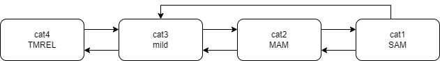
Our transition model of child wasting will consist of the same 4 GBD risk exposure categories as the GBD child wasting model. In our transition model, simulants may transition between adjacent categories as well as between the cat1 (SAM) and cat3 (mild) categories, representing a pathway for those successfully treated for SAM.
Risk exposure model diagram
Important
The modeling strategy on this page applies to all simulants from birth to 5 years of age for use in wave II of the nutrition optimization model. Note that this is a change from the wave I strategy, described in the note below.
Note
For wave I of the nutrition optimization model:
We will modeled wasting transitions as detailed on this page only among simulants at least six months of age.
For wave I, infants 0-6 months followed the Static wasting exposure modeling strategy.
Initialization
Simulants will be initialized into a wasting state at birth according to the wasting risk exposure distribution specific to the 1-5 month (ID 388) age group.
Wasting state at initialization will be entirely dependent on infant LBWSG exposure, such that low birth weight (LBW) infants with birth weight exposures equal to or below 2,500 grams will have a greater probability of being wasted than adequate birth weight (ABW) infants with birth weight exposures greater than 2,500 grams.
Parameter |
Definition |
Note |
|---|---|---|
\(p_\text{cat(i)}\) |
Population level prevalence of wasting category i |
In the 1-5 month age group (ID=388) |
\(p_\text{cat(i),LBW}\) |
Prevalence of wasting category i among the low birth weight population |
Low birth weight as BW =< 2,500 grams |
\(p_\text{cat(i),ABW}\) |
Prevalence of wasting catgory i among the adequate birth weight population |
Adequate birth weight as BW > 2,500 grams |
RR |
Relative risk of wasting (cat1 and cat2 combined) at 30 days of life among LBW relative to ABW babies |
|
\(p_\text{LBW}\) |
Prevalence of low birth weight among infants who survive to 30 days of life |
This value is specific to the baseline scenario |
Given the following equations:
\(p_\text{cat1,LBW} * p_\text{LBW} + p_\text{cat1,ABW} * (1 - p_\text{LBW}) = p_\text{cat1}\)
\(RR = p_\text{cat1,LBW} / p_\text{cat1,ABW}\)
We can then solve for the ABW and LBW probabilities of initialization into wasting categories 1 and 2. We then assume that the difference between the ABW and LBW probabilities for categories 1 and 2 with the population-level probabilities is equally distributed amongst categories 3 and 4.
Wasting category |
ABW probability |
LBW probability |
|---|---|---|
cat1 |
\(p_\text{cat1} / (RR * p_\text{LBW} + (1 - p_\text{LBW}))\) |
\(p_\text{ABW,cat1} * RR\) |
cat2 |
\(p_\text{cat2} / (RR * p_\text{LBW} + (1 - p_\text{LBW}))\) |
\(p_\text{ABW,cat2} * RR\) |
cat3 |
\((p_\text{cat1} + p_\text{cat2} - p_\text{ABW,cat1} - p_\text{ABW,cat2}) * p_\text{cat3} / (p_\text{cat3} + p_\text{cat4}) + p_\text{cat3}\) |
\((p_\text{cat1} + p_\text{cat2} - p_\text{LBW,cat1} - p_\text{LBW,cat2}) * p_\text{cat3} / (p_\text{cat3} + p_\text{cat4}) + p_\text{cat3}\) |
cat4 |
\((p_\text{cat1} + p_\text{cat2} - p_\text{ABW,cat1} - p_\text{ABW,cat2}) * p_\text{cat4} / (p_\text{cat3} + p_\text{cat4}) + p_\text{cat4}\) |
\((p_\text{cat1} + p_\text{cat2} - p_\text{LBW,cat1} - p_\text{LBW,cat2}) * p_\text{cat4} / (p_\text{cat3} + p_\text{cat4}) + p_\text{cat4}\) |
Note
The values in the Wasting state probabilities by birth weight status should not change between scenarios as LBWSG exposures change.
Todo
Update placeholder values below
Parameter |
Value |
Note/Source |
|---|---|---|
RR |
1.82 (95% CI: 1.35, 2.45), assume a lognormal distribution of uncertainty |
Calculated using meta-analysis of most recent available DHS round 7 or 8 as of 10/2023. Analysis performed and resulting forest plot can be found here |
\(p_\text{LBW}\) |
|
LBWSG exposure document found here for reference. List of LBW categories was generated from this notebook |
Note that prevalence of each wasting state for use in this model can be pulled using the following call:
get_draws(gbd_id_type='rei_id',
                gbd_id=240,
                source='exposure',
                year_id=2021,
                gbd_round_id=7,
                decomp_step='iterative')
Transitions
Draw-specific values for transition rates (defined in the table below) for Ethiopia, Nigeria, and Pakistan (GBD 2019 cause data and GBD 2021 CGF data for use in Nutrition Optimization Wave I) can be found listed below. Values in these files are defined in terms of transitions per person-year in the source state.
Transition |
Source State |
Sink State |
|---|---|---|
ux_rem_rate_sam |
CAT 1 |
CAT 2 |
tx_rem_rate_sam |
CAT 1 |
CAT 3 |
rem_rate_mam |
CAT 2 |
CAT 3 |
rem_rate_mild |
CAT 3 |
CAT 4 |
inc_rate_sam |
CAT 2 |
CAT 1 |
inc_rate_mam |
CAT 3 |
CAT 2 |
inc_rate_mild |
CAT 4 |
CAT 3 |
MAM (cat2) substates
Note
This was implemented in a manner that divided the MAM state into two separate states, creating an overall 5-category wasting transition model. Transition rates from the 4-category model were scaled such that transitions in and out of the MAM category did not vary by MAM substate.
For simulants that transition into the moderate acute malnutrition (MAM, cat2) wasting exposure state, they will be assigned one of the two following sub-exposures:
“Better” MAM/cat2.5: WHZ between -2 and -2.5
“Worse” MAM/cat2.0: WHZ between -2.5 and -3
The probability of occupying the “Worse” MAM/cat2.0 sub-exposure upon transitioning into the MAM state is can be found in this CSV file. The probability of “Better” MAM/cat2.5 is equal to 1-the probability of Worse MAM.
These probabilities were generated according to a continuous distribution of child WHZ scores, as performed in this notebook. Note that mean WHZ and WHZ sd estimates from GBD were not available for GBD 2021, so we used DHS data to inform these parameters paired with GBD ensemble distribution weights to generate a continuous WHZ distribution for this purpose.
In April of 2024, this was updated due to a found bug in the code. The data was aggregated over age and sex, though kept location specific. The data file and notebook were updated accordingly. This change was due to lack of difference at the age or sex level, and small counts leading to NaN values and incorrect final data.
These subexposures will vary with respect to their wasting relative risk values (detailed on the CGF risk effects page) and their targeted MAM treatment eligibility (detailed on the wasting treatment page), but they will not differ with respect to wasting transition rates (e.g. progression to SAM or recovery to mild wasting states).
Note
These sub-exposures should be included in wasting state person-time observers.
Validation
Wasting model
prevalence of cat 1-4 (including the MAM sub-states)
model transition rates
Note that validation of this model is dependent on validation of wasting-specific mortality rates, which are dependent on the following models meeting their individual validation criteria:
Stunting and underweight exposure models
CGF risk exposure correlation
CGF risk effects
Cause-specific and all-cause mortality rates
Deriving the wasting transition rates
We utilized information from several sources to develop a wasting transition model.
Wasting risk exposure: GBD 2021 risk prevalence
Wasting-specific mortality rates:
GBD 2019 cause models for diarrheal diseases, lower respiratory infections, measles, and malaria (as linked on the nutrition optimization child concept model)
Treated MAM and SAM recovery rates: wasting treatment intervention model
Incidence rates from less to more severe wasting categories: BMGF Knowledge Integration (KI) longitudinal database. A description of included studies is available here
However, recovery from MAM and SAM states for those who do not receive treatment is very limited in the case of MAM and not observable in the case of SAM as it would be unethical for researchers to track the natural history of SAM without providing access to treatment. Therefore, we utilized a Markov model to solve for the untreated wasting recovery rates that would result in a steady state equilibrium of the system below and the values from the sources described above.
Note
The previous implementation of this model relied on literature estimates of untreated recovery rates from SAM and MAM (observed indirectly in the case of untreated SAM) and used the markov steady state model to solve for wasting incidence rates. This update is an improvement upon the previous implementation in that it relies on directly observed data as inputs to the model and outputs values for limited/un-observable parameters rather than the other way around. Additionally, this implementation results in values that better validate to KI transition rate data where applicable.

A small-level individual-based simulation has demonstrated the system of equations used in the derivation of these rates successfully maintains steady state. See a demonstration of the steady state equilibrium maintained by this system of equations in this notebook
The process of generating draw-level values for all wasting transitions is outlined below. See the code for generating draw-specific transition values in this notebook here
Load all input data values (in accordance with documentation linked above)
Exclude studies in the KI database that have inappropriate study populations. A list of excluded studies and there reasons for exclusion are provided below.
AKU_EE: Infants with insufficient response to RUTF
DIVIDS: Small for gestational age infants, not SAM, not ill
Ilins-Dose: LNS supplementation
Ilins-Dyad: LNS supplementation
SAS_LBW: LBW babies
At the sex, age, and draw-specific level, randomly sample a study from the remaining KI studies
Randomly sample event count values (numerator values) for i1, i2, and i3 transition rates under the assumption that the event counts follow a Poisson distribution of uncertainty, divide by person-time denominators (child days in provided KI data), and then convert to daily transition probabilities
Calculate r4, r3 (as well as r3_treated and r3_untreated), r2 recovery probabilities according to draw-specific input parameters and sampled i1, i2, and i3 values
Assess validity of results according to the following rules:
r4, r3, r3_untreated, and r2 must be positive
t1 must be greater than r2
r3_treated must be greater than r3_untreated
result for r3 value solved by two different methods must be within 10% of one another
If any of the rules in step #6 fail, begin again at step #3 until valid result is obtained. Repeat until 1,000 valid draws are generated for each age/sex group
Convert daily probabilities to annual rates and output as .csv
Assumptions and Limitations
We do not consider seasonal variation in wasting exposure or transition rates
We do not consider individual heterogeneity in wasting transition rates beyond what is modeled in the wasting x-factor model when it is included in the simulation
We rely on treatment data with sparse availability and assume that child wasting measured by WHZ is a reasonable proxy for acute malnutrition (often measured by MUAC)
We cannot directly observe recovery time of untreated wasting as it would be unethical. Therefore, we must indirectly estimate this parameter
We assume that those successfully treated for SAM transition directly to the mild wasting state without transitioning through the MAM state. By definition, a transition through the MAM state must occur in reality. However, this design was selected for convenient compatibility with the standard discharge criteria for SAM treatment used in studies that report treated SAM recovery rates. Additionally, there is some data to suggest that immunologic recovery (and therefore reduction in mortality risk) of SAM cases lags behind anthropomorphic recovery.
References
Todo
Link GBD 2021 methods appendix when finished