Risk Effects
What is a risk effect?
A risk effect is a measure of how some variable (the risk factor) causally impacts some outcome variable.
Generally, we will use risk effects models to represent a causal effect of one variable on another and risk correlation models to represent non-causal associations between two variables (see the causality documentation page for more information on causality). It is important to note that for any two variables that are causally related to one another, there is likely also additional non-causal correlation between them through additional variables and shared common causes.
There are several attributes of a risk effect that are important to consider, including the
direction (ex: positive or negative effect of increased exposure),
shape (ex: linear, U-shaped, etc.),
magnitude (ex: large or small),
and statisical certainty
of the effect the risk factor has on the outcome.
The risk effect may be measured in both absolute (ex: risk difference) or relative terms (ex: relative risk). See the measures of risk page for more information on such measures.
To implement a risk effect in simulation we also need to know how to delete that effect from baseline population-level rates of the outcome. This is done with a measure of population impact.
Risk effects in GBD
GBD reports risk effects using relative risks (RRs) and population attributable fractions (PAFs). A relative risk describes the multiplier on the risk of the outcome caused by exposure.
For GBD risk factors with categorical risk exposures, GBD reports an estimated relative risk for each level of risk exposure, relative to the TMREL for that risk.
For most GBD risk factors with continuous risk exposures (see below for exceptions starting in GBD 2021), GBD reports an estimated relative risk caused by each increase of a specified amount in risk exposure above the TMREL. This specified increase may be more than a single unit change in risk exposure, so it is important to clarify this with the GBD modeler.
Todo
Determine if there is a data source that documents these units
GBD risk effects are typically estimated by meta-analysis of epidemiologic studies that assess how different levels of risk exposures affect some outcome variable such as an incidence or mortality rate. There are several factors that may bias the quantification of a risk effect in epidemiologic studies (including influence by confounding), and causal inference from such studies may be inhibited by such limitations. See the page on causality for more information on the topic.
The GBD-estimated relative risks are assumed to represent the causal effect of the risk on the outcome, as they are calculated in the absense of confounding factors and the evidence is assessed to ensure it meets criteria for causality. See the causality documentation page for more information on the topic. GBD has begun to quantify the quality of evidence for causality between risk-outcome pairs they model in an effort termed “the burden of proof,” summarized in publications such as [Zheng-et-al-2022] and this webpage. Additionally, the GBD-estimated relative risks represent the total effect of the risk on the outcome, including any mediated effects. See the mediation documentation page for more information on the topic.
While relative risks in GBD are typically age- and sex-specific, they are assumed not to vary by location or year. GBD applies risk effects to either YLDs, YLLs, or both. Importantly, a risk factor could affect YLDs due to a given condition by affecting its incidence rate, remission rate, or severity of disease. Therefore, it is important to discuss reasonable assumptions with subject matter experts to determine the most appropriate measure to which to apply the GBD risk effects in our vivarium simulations.
Starting in GBD 2021, some continuous risk exposures were modeled with general relationships between the exposure level and the relative risk (going beyond the log-linear relationship assumed for previous iterations). Interpreting the GBD estimates is straightforward, once you have chased down all of the necessary definitions. The relevant estimates include a column for exposure level, as well as columns for 500 draws of relative risk values at each exposure level. These represent points on the continuous curve, which can then be approximated by interpolating these points. The GBD 2021 PAF calculator often selected a TMREL for each draw from a uniform distribution, but for some risk factors, analysts provided draws for the TMREL as well. The precise calculation to go from exposure levels and GBD-recorded risks to a function suitable for use as \(f_{rr}\) as defined below are perhaps most clearly represented as python code:
import numpy as np
import scipy.interpolate
import matplotlib.pyplot as plt
import gbd_mapping, vivarium_gbd_access.gbd

# Replace with your risk of interest
risk = gbd_mapping.risk_factors.high_systolic_blood_pressure
# Replace with your cause of interest
cause = gbd_mapping.causes.ischemic_heart_disease
age_group_id = 20 # 75 to 79
sex_id = 1 # Male
year_id = 2021

relative_risk_data = vivarium_gbd_access.gbd.get_relative_risk(
    risk.gbd_id,
    1, # Global
    year_id=year_id,
)

# Subset to cause, age, and sex of interest
# If interested in multiple, would loop through them
relative_risk_data = relative_risk_data[
    (relative_risk_data.cause_id == cause.gbd_id) &
    (relative_risk_data.age_group_id == age_group_id) &
    (relative_risk_data.sex_id == sex_id)
].sort_values('exposure')

relative_risk_functions = {}

# Do calculation at the draw level
for draw_id in range(1_000):
    relative_risk_draw = relative_risk_data[f'draw_{draw_id}']
    # interpolate a continuous function between the points,
    # and extrapolate outside the range with the endpoints
    raw_relative_risk_function = scipy.interpolate.interp1d(
        relative_risk_data.exposure,
        relative_risk_draw,
        kind='linear',
        bounds_error=False,
        fill_value=(
            relative_risk_draw.min(),
            relative_risk_draw.max(),
        )
    )

    # pick a tmrel between tmred.min and tmred.max and calculate relative risk at tmrel
    # for certain risk factors, the modeling team uploads a model for this with TMREL draws --
    # those should be used instead of this, when available!
    tmrel = np.random.uniform(risk.tmred.min, risk.tmred.max)
    rr_at_tmrel = raw_relative_risk_function(tmrel)
    normalized_relative_risk_draw = relative_risk_draw / rr_at_tmrel

    # This clipping is what the GBD PAF calculator does, but it is not clear that it makes
    # sense conceptually.
    # A single risk factor can have positive (protective) and negative (harmful) effects on
    # different causes, and the TMREL can then be a balance between them, which doesn't necessarily
    # imply it is the ideal exposure when looking at either cause individually.
    # TODO: Revisit this.
    clipped_normalized_relative_risk_draw = np.clip(normalized_relative_risk_draw, 1.0, np.inf)

    relative_risk_function = scipy.interpolate.interp1d(
        relative_risk_data.exposure,
        clipped_normalized_relative_risk_draw,
        kind='linear',
        bounds_error=False,
        fill_value=(
            clipped_normalized_relative_risk_draw.min(),
            clipped_normalized_relative_risk_draw.max(),
        )
    )

    relative_risk_functions[draw_id] = relative_risk_function

# Plot the relative risk functions
x_values = np.linspace(relative_risk_data.exposure.min() * 0.5, relative_risk_data.exposure.max() * 1.5, 500)
mean = np.zeros_like(x_values)

for i, function in enumerate(relative_risk_functions.values()):
    y_values = function(x_values)
    plt.plot(x_values, y_values, color="gray", alpha=0.01)
    mean += y_values

mean = mean / len(relative_risk_functions)
plt.plot(x_values, mean, color="green")
plt.gca().set_xlabel(f'{risk.name} exposure')
plt.gca().set_ylabel(f'RR of {cause.name}')
plt.show()
This code generates a separate function/curve for each draw, as seen in the plot:
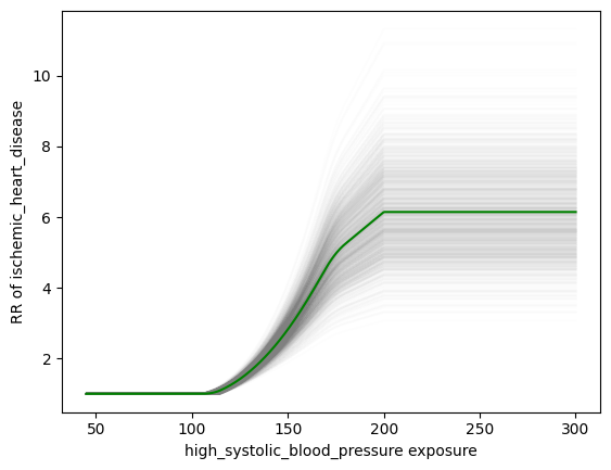
We’ve validated that using this approach, we can get approximately the same result as the GBD PAF calculator. The relevant code in the PAF calculator is on Stash; the clipping is implemented here. This is demonstrated in this notebook.
Finally, it is important to note that because the GBD relative risks represent the causal impact between and risk and an outcome, they cannot represent the non-causal association between a given risk and an outcome or other risk factors. Desired correlation between two variables will need to be accounted for separately; see the risk correlation page for more details.
Risk effects in Vivarium
Materials related to risk effects models in Vivarium:
Generally, we will use risk effects models to represent causal associations between two variables and risk correlation models to represent non-causal associations between two variables in vivarium.
In Vivarium, we build risk effect components in order to study the impact on outcomes of interest contributed by a given risk exposure. The outcome might be a cause (e.g. ischemic heart disease attributable to high body-mass index) or a intermediate outcome (e.g. systolic blood pressure associated with BMI). For a risk-cause pair, our risk effects models typically link the incidence (or other measure such as excess mortality rate) of that cause to the exposure of the risk.
A risk effects model for a given risk-outcome pair must document:
Relative risk as a function of risk exposure.
Instructions for how to delete the baseline effect.
You can think of deleting the baseline effect as finding the outcome rate for simulants with the lowest-risk exposure. The outcome rate estimated by GBD at the population level is across the population distribution of exposure, so the effect of the risk exposure on the outcome is already partially baked into that population-level number. Deleting the effects of baseline exposure yields the outcome rate in a counterfactual where everyone is at the lowest-risk exposure, which we assign to all simulants before applying their exposure-specific risk effect. We delete the baseline effect with a measure of population impact.
- The mathematical expressions mainly fall into two categories:
- risk exposure is categorical:
\(i_{exposed} = i \times (1-PAF) \times RR\)
\(i_{unexposed} = i \times (1-PAF)\)
\(PAF = \frac{E(RR_e)-1}{E(RR_e)}\)
\(E(RR_e) = p \times RR + (1-p)\)
- risk exposure is continuous:
- risk effect has a log-linear “dose-response” relationship with exposure:
\(i_{\text{simulant}} = i \times (1-PAF) \times rr^{max(e_{\text{simulant}}-tmrel,0)/scalar}\)
\(PAF = \frac{E(RR_e)-1}{E(RR_e)}\)
\(E(RR_e) = \int_{lower}^{upper}rr^{max(e-tmrel,0)/scalar}p(e)de\)
- risk effect has a non-log-linear relationship with exposure:
\(i_{\text{simulant}} = i \times (1-PAF) \times f_{rr}(e_{\text{simulant}})\)
\(PAF = \frac{E(RR_e)-1}{E(RR_e)}\)
\(E(RR_e) = \int_{lower}^{upper}f_{rr}(e)p(e)de\)
- Where,
\(e\) stands for risk exposure level
\(i\) stands for incidence rate
\(p\) stands for proportion of exposed population
\(RR\) stands for relative risk or incidence rate ratio
\(PAF\) stands for population attributable fraction (described in detail here)
\(E(RR_e)\) stands for expected relative risk at risk exposure level e
\(tmrel\) stands for theoretical minimum risk exposure level
\(lower\) stands for minimum exposure value
\(upper\) stands for maximum exposure value
\(rr\) is the base of the exponent in an exponential relative risk model
\(scalar\) is a numeric variable used to convert risk exposure level to a desired unit
\(p(e)\) is probability density function used to calculate the probability of given risk exposure level e
\(f_{rr}(e)\) is function capturing the relationship between the exposure level and the relative risk at that exposure level (for log-linear relative risks, \(f_{rr}(e) = rr^{max(e-tmrel,0)/scalar}\)) of given risk exposure level e
We can refer to the outcome rate multiplied by (1 - PAF) as the “risk-deleted outcome rate.”
Using RRs and PAFs from GBD
While GBD reports RRs and PAFs, they are often not suitable for use in Vivarium models. This is because we typically model GBD causes as dynamic state-transition models, and are interested in applying RRs and PAFs to transitions in the model, while GBD’s RRs and PAFs are applied to static, population level quantities, namely years of life lost (YLLs) and years lived with disability (YLDs).
YLLs are the number of deaths (due to a cause) multiplied by the average remaining life expectancy (which is a constant for a given age and sex group). The number of deaths due to a cause is that cause’s cause-specific mortality rate (CSMR) multiplied by the population size, which is also a constant for a given age and sex group. YLDs are the number of prevalent cases of a cause multiplied by the disability weight of that cause, which is a constant for a given cause. Therefore, since relative risk is computed as a ratio (and the PAF is computed from the RRs), the constant factors cancel out, and we get
However, if we have a dynamic SIS model for a cause, we are interested in applying risk effects to the transitions in this diagram:
The RR and PAF we have on prevalence (aka the number of people in the infected state) might apply to either of the incidence and remission transition rates, or some combination. Intuitively, the fact that more people with the risk exposure have the disease might be because more of them get the disease, or because it takes longer for them to recover from it.
Note
Technically, mortality also matters: if the risk exposure causes people to die more quickly if they have the disease, that will lower the effect of the risk exposure on prevalence (since people who die are no longer prevalent cases). However, this effect is small when the mortality rate overall is small. See TODO below to make this precise.
We typically apply the risk effect to the incidence rate, but this is a modeling choice. With this choice:
The RR and PAF we have on CSMR doesn’t directly fit anywhere into our diagram, because CSMR is a mortality rate among the total population, and our mortality transition only applies to the infected population. Intutively, the CSMR RR is partially overlapping with the prevalence RR; there could be more deaths among people with the risk exposure because they are more likely to have the disease, even if they are no more likely to die from it once they have it.
We’ve developed a simple equation to adjust the CSMR RR to apply to the excess mortality rate:
Note
In this equation, which we calculate at the draw level, we act as though the covariance between \(RR_\text{CSMR}\) and \(RR_\text{incidence}\) has been estimated by GBD.
However, it hasn’t been, and these quantities will be independent at the draw level, though we would intuitively expect a strong correlation.
Primarily due to this independence assumption, the equation above will in some draws result in an \(RR_\text{excess mortality} < 1\). This is not conceptually incoherent (perhaps a risk factor could cause more cases, but they are on average less severe and less likely to cause death) but probably happens far too often due to the independence issue.
The larger covariance issue is tracked at: https://jira.ihme.washington.edu/browse/SSCI-2161
The PAF on excess mortality has no such simple approximation, so should be recalculated from the new RR using the relevant equation (for the categorical or continuous case) from the top of this section. (For a more explicit description of this process, but with the added complication of handling multiple risk factors at once, see Calculation of joint PAFs in presence of correlation. As noted there, we do not yet have a standard computational approach to calculating our own PAFs.)
Todo
Make this precise. I believe that this is heuristic and not quite correct. The child growth failure risk effects page includes a notebook that approximately checks it numerically, and a Word document that concludes with an “almost identical” equation that seems importantly different. Also, the Word doc appears to be about a risk factor that affects mortality, rather than a risk factor that affects a disease that affects mortality? So I think something has been lost here. See https://jira.ihme.washington.edu/browse/SSCI-2160.
Todo
Add a note about bias this introduces…
PAF relies on exposure in the population, not the “at-risk” group for the outcome. This bias is larger when the at-risk population is small relative to the total population.
But maybe this belongs in the PAF section?
Relevant ticket in backlog: https://jira.ihme.washington.edu/browse/SSCI-1152
Restrictions
As with cause models, risk effects models may include restrictions, which answer the questions: Who does this apply to? For which population groups (e.g., age or sex group) is this risk effect not valid?
It is worth noting that although risk effect and risk exposure both are related to risk factors, restrictions for these two elements function differently. Risk exposure restrictions do not include outcome restrictions (i.e., YLL only or YLD only), however risk effect restrictions do. Due to the nature of the relationship between risk exposure and risk effects, risk effects restrictions will always be within restrictions for risk exposure. To illustrate, if a risk exposure restriction for a given risk factor is male only, then the risk effects model will also be restricted to male only.
For example, GBD 2019 modeled low-birthweight and short gestation (LBWSG) relative risks with age and outcome restrictions. See the table below for details.
Restriction Type |
Value |
Notes |
|---|---|---|
Male only |
False |
|
Female only |
False |
|
YLL only |
True |
Except for Neonatal preterm birth; see note below |
YLD only |
False |
|
Age group start |
Early neonatal (0-7 days, age_group_id = 2) |
|
Age group end |
Late neonatal (7-28 days, age_group_id = 3) |
Except for Neonatal preterm birth; see note below |
Note
GBD attributes 100% of the DALYs due to Neonatal Preterm Birth to the LBWSG risk factor. In particular, the attribution includes YLDs as well as YLLs, and the age restrictions for the LBWSG-attributable DALYs are the same as the age restrictions for Neonatal Preterm Birth.
YLLs due to Neonatal preterm birth, 100% attributable to LBWSG:
Age group start = 2 (Early neonatal, 0-7 days)
Age group end = 5 (1 to 4)
YLDs due to Neonatal preterm birth, 100% attributable to LBWSG:
Age group start = 2 (Early neonatal, 0-7 days)
Age group end = 235 (95+)
Note that this attribution of DALYs is not based on the relative risks for all-cause mortality, but instead is based on the logic that all preterm births are due to short gestation by definition. Thus, if we include Neonatal Preterm Birth in our models, the relative risks likely must be handled differently for this cause.
Todo
Follow up about assumptions that GBD uses to apply relative risk to YLLs and YLDs.